Infinitesimal sequences – definition and properties. Examples What quantity is called infinitesimal

Calculus of infinitesimals and larges

Infinitesimal calculus- calculations performed with infinitesimal quantities, in which the derived result is considered as an infinite sum of infinitesimals. The calculus of infinitesimals is a general concept for differential and integral calculus, which forms the basis of modern higher mathematics. The concept of an infinitesimal quantity is closely related to the concept of limit.

Infinitesimal

Subsequence a n called infinitesimal, If . For example, a sequence of numbers is infinitesimal.

The function is called infinitesimal in the vicinity of a point x 0 if .

The function is called infinitesimal at infinity, If or .

Also infinitesimal is a function that is the difference between a function and its limit, that is, if , That f(x) − a = α( x) , .

Infinitely large quantity

In all the formulas below, infinity to the right of equality is implied to have a certain sign (either “plus” or “minus”). That is, for example, the function x sin x, unbounded on both sides, is not infinitely large at .

Subsequence a n called infinitely large, If .

The function is called infinitely large in the vicinity of a point x 0 if .

The function is called infinitely large at infinity, If or .

Properties of infinitely small and infinitely large

Comparison of infinitesimals

How to compare infinitesimal quantities?
The ratio of infinitesimal quantities forms the so-called uncertainty.

Definitions

Suppose we have infinitesimal values α( x) and β( x) (or, which is not important for the definition, infinitesimal sequences).

To calculate such limits it is convenient to use L'Hopital's rule.

Comparison examples

Using ABOUT-symbolism, the results obtained can be written in the following form x 5 = o(x 3). In this case, the following entries are true: 2x 2 + 6x = O(x) And x = O(2x 2 + 6x).

Equivalent values

Definition

If , then the infinitesimal quantities α and β are called equivalent ().
It is obvious that equivalent quantities are a special case of infinitesimal quantities of the same order of smallness.

When the following equivalence relations are valid (as consequences of the so-called remarkable limits):

Theorem

The limit of the quotient (ratio) of two infinitesimal quantities will not change if one of them (or both) is replaced by an equivalent quantity.

This theorem has practical significance when finding limits (see example).

Usage example

Replacing sin 2x equivalent value 2 x, we get

Historical sketch

The concept of “infinitesimal” was discussed back in ancient times in connection with the concept of indivisible atoms, but was not included in classical mathematics. It was revived again with the advent of the “method of indivisibles” in the 16th century - dividing the figure under study into infinitesimal sections.

In the 17th century, the algebraization of infinitesimal calculus took place. They began to be defined as numerical quantities that are less than any finite (non-zero) quantity and yet not equal to zero. The art of analysis consisted in drawing up a relation containing infinitesimals (differentials) and then integrating it.

Old school mathematicians put the concept to the test infinitesimal harsh criticism. Michel Rolle wrote that the new calculus is “ set of ingenious mistakes"; Voltaire caustically remarked that calculus is the art of calculating and accurately measuring things whose existence cannot be proven. Even Huygens admitted that he did not understand the meaning of differentials of higher orders.

As an irony of fate, one can consider the emergence in the middle of the century of non-standard analysis, which proved that the original point of view - actual infinitesimals - was also consistent and could be used as the basis for analysis.

So, let’s fix an arbitrary number ε > 0. Since according to the conditions of the theorem α(x) is an infinitesimal function, then there is such δ 1 > 0, which is |x – a|< δ 1 we have |α(x)|< ε / 2. Likewise, since β(x) is infinitesimal, then there is such δ 2 > 0, which is |x – a|< δ 2 we have | β(x)|< ε / 2.

Let's take δ=min(δ 1 , δ2 } .Then in the neighborhood of the point a radius δ each of the inequalities will be satisfied |α(x)|< ε / 2 and | β(x)|< ε / 2. Therefore, in this neighborhood there will be

|f(x)|=| α(x)+β(x)| ≤ |α(x)| + | β(x)|< ε /2 + ε /2= ε,

those. |f(x)|< ε, which is what needed to be proved.

Theorem 2. Product of an infinitesimal function a(x) for a limited function f(x) at x→a(or when x→∞) is an infinitesimal function.

Proof. Since the function f(x) is limited, then there is a number M such that for all values x from some neighborhood of a point a|f(x)|≤M. Moreover, since a(x) is an infinitesimal function at x→a, then for an arbitrary ε > 0 there is a neighborhood of the point a, in which the inequality will hold |α(x)|< ε /M. Then in the smaller of these neighborhoods we have | αf|< ε /M= ε. And this means that af– infinitesimal. For the occasion x→∞ the proof is carried out similarly.

From the proven theorem it follows:

Corollary 1. If and, then.

Corollary 2. If c= const, then .

Theorem 3. Ratio of an infinitesimal function α(x) per function f(x), whose limit is different from zero, is an infinitesimal function.

Proof. Let . Then 1 /f(x) there is a limited function. Therefore the fraction is the product of an infinitesimal function and a bounded function, i.e. function is infinitesimal.

RELATIONSHIP BETWEEN INFINITELY SMALL AND INFINITELY LARGE FUNCTIONS

Theorem 1. If the function f(x) is infinitely large at x→a, then function 1 /f(x) is infinitesimal at x→a.

Proof. Let's take an arbitrary number ε >0 and show that for some δ>0 (depending on ε) for all x, for which |x – a|<δ , the inequality is satisfied, and this will mean that 1/f(x) is an infinitesimal function. Indeed, since f(x) is an infinitely large function at x→a, then there will be δ>0 such that as soon as |x – a|<δ , so | f(x)|> 1/ ε. But then for the same x.

Examples.

The converse theorem can also be proven.

Theorem 2. If the function f(x)- infinitesimal at x→a(or x→∞) and does not vanish, then y= 1/f(x) is an infinitely large function.

Conduct the proof of the theorem yourself.

Examples.

Thus, the simplest properties of infinitesimal and infinitely large functions can be written using the following conditional relations: A≠ 0

LIMIT THEOREMS

Theorem 1. The limit of the algebraic sum of two, three, and generally a certain number of functions is equal to the algebraic sum of the limits of these functions, i.e.

Proof. Let us carry out the proof for two terms, since it can be done in the same way for any number of terms. Let .Then f(x)=b+α(x) And g(x)=c+β(x), Where α And β – infinitesimal functions. Hence,

f(x) + g(x)=(b + c) + (α(x) + β(x)).

Because b+c is a constant, and α(x) + β(x) is an infinitesimal function, then

Example. .

Theorem 2. The limit of the product of two, three, and generally a finite number of functions is equal to the product of the limits of these functions:

Proof. Let . Hence, f(x)=b+α(x) And g(x)=c+β(x) And

fg = (b + α)(c + β) = bc + (bβ + cα + αβ).

Work bc there is a constant value. Function bβ + c α + αβ based on the properties of infinitesimal functions, there is an infinitesimal quantity. That's why .

Corollary 1. The constant factor can be taken beyond the limit sign:

Corollary 2. The degree limit is equal to the limit degree:

Example..

Theorem 3. The limit of the quotient of two functions is equal to the quotient of the limits of these functions if the limit of the denominator is different from zero, i.e.

Proof. Let . Hence, f(x)=b+α(x) And g(x)=c+β(x), Where α, β – infinitesimal. Let's consider the quotient

A fraction is an infinitesimal function because the numerator is an infinitesimal function and the denominator has a limit c 2 ≠0.

Examples.

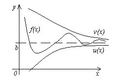
Theorem 4. Let three functions be given f(x), u(x) And v(x), satisfying the inequalities u (x)≤f(x)≤ v(x). If the functions u(x) And v(x) have the same limit at x→a(or x→∞), then the function f(x) tends to the same limit, i.e. If

, That .

The meaning of this theorem is clear from the figure.

The proof of Theorem 4 can be found, for example, in the textbook: Piskunov N. S. Differential and integral calculus, vol. 1 - M.: Nauka, 1985.

Theorem 5. If at x→a(or x→∞) function y=f(x) accepts non-negative values y≥0 and at the same time tends to the limit b, then this limit cannot be negative: b≥0.

Proof. We will carry out the proof by contradiction. Let's pretend that b<0 , Then |y – b|≥|b| and, therefore, the difference modulus does not tend to zero when x→a. But then y does not reach the limit b at x→a, which contradicts the conditions of the theorem.

Theorem 6. If two functions f(x) And g(x) for all values of the argument x satisfy the inequality f(x)≥ g(x) and have limits, then the inequality holds b≥c.

Proof. According to the conditions of the theorem f(x)-g(x) ≥0, therefore, by Theorem 5 , or .

UNILATERAL LIMITS

So far we have considered determining the limit of a function when x→a in an arbitrary manner, i.e. the limit of the function did not depend on how it was located x towards a, to the left or right of a. However, it is quite common to find functions that have no limit under this condition, but they do have a limit if x→a, remaining on one side of A, left or right (see figure). Therefore, the concepts of one-sided limits are introduced.

If f(x) tends to the limit b at x tending to a certain number a So x accepts only values less than a, then they write and call blimit of the function f(x) at point a on the left.

Calculus of infinitesimals and larges

Infinitesimal

Subsequence a n called infinitesimal, If . For example, a sequence of numbers is infinitesimal.

The function is called infinitesimal in the vicinity of a point x 0 if .

The function is called infinitesimal at infinity, If or .

Also infinitesimal is a function that is the difference between a function and its limit, that is, if , That f(x) − a = α( x) , .

Infinitely large quantity

Subsequence a n called infinitely large, If .

The function is called infinitely large in the vicinity of a point x 0 if .

The function is called infinitely large at infinity, If or .

In all cases, infinity to the right of equality is implied to have a certain sign (either “plus” or “minus”). That is, for example, the function x sin x is not infinitely large at .

Properties of infinitely small and infinitely large

Comparison of infinitesimals

How to compare infinitesimal quantities?
The ratio of infinitesimal quantities forms the so-called uncertainty.

Definitions

Suppose we have infinitesimal values α( x) and β( x) (or, which is not important for the definition, infinitesimal sequences).

To calculate such limits it is convenient to use L'Hopital's rule.

Comparison examples

Using ABOUT-symbolism, the results obtained can be written in the following form x 5 = o(x 3). In this case, the following entries are true: 2x 2 + 6x = O(x) And x = O(2x 2 + 6x).

Equivalent values

Definition

If , then the infinitesimal quantities α and β are called equivalent ().
It is obvious that equivalent quantities are a special case of infinitesimal quantities of the same order of smallness.

When the following equivalence relations are valid: , , .

Theorem

The limit of the quotient (ratio) of two infinitesimal quantities will not change if one of them (or both) is replaced by an equivalent quantity.

This theorem has practical significance when finding limits (see example).

Usage example

Replacing sin 2x equivalent value 2 x, we get

Historical sketch

Disputes in the Paris Academy of Sciences regarding the justification of analysis became so scandalous that the Academy once completely forbade its members to speak on this topic (this mainly concerned Rolle and Varignon). In 1706 Rolle publicly withdrew his objections, but discussions continued.

In 1734, the famous English philosopher, Bishop George Berkeley, published a sensational pamphlet, known under the abbreviated title “ Analyst" Its full name: " An Analyst or Discourse addressed to the unbelieving mathematician, inquiring whether the subject, principles, and conclusions of modern analysis are more clearly perceived or more clearly deduced than the religious mysteries and articles of faith».

The Analyst contained a witty and largely fair criticism of infinitesimal calculus. Berkeley considered the method of analysis to be inconsistent with logic and wrote that, “ however useful it may be, it can only be considered as a kind of guess; deft skill, art or rather trick, but not as a method of scientific proof" Quoting Newton’s phrase about the increment of current quantities “at the very beginning of their origin or disappearance,” Berkeley ironically: “ they are neither finite quantities, nor infinitesimals, nor even nothing. Could we not call them the ghosts of deceased magnitudes?... And how can we generally talk about the relationship between things that do not have magnitude?.. Anyone who can digest the second or third fluxion [derivative], the second or third difference, should not, as it seems to me to find fault with something in theology».

It is impossible, writes Berkeley, to imagine instantaneous speed, that is, speed at a given instant and at a given point, because the concept of motion includes the concepts of (finite non-zero) space and time.

How does analysis produce correct results? Berkeley came to the idea that this was explained by the presence of several errors in the analytical conclusions, and illustrated this with the example of a parabola. It is interesting that some major mathematicians (for example, Lagrange) agreed with him.

A paradoxical situation arose when rigor and fruitfulness in mathematics interfered with each other. Despite the use of illegal actions with poorly defined concepts, the number of direct errors was surprisingly small - intuition came to the rescue. And yet, throughout the 18th century, mathematical analysis developed rapidly, without essentially any justification. Its efficiency was amazing and spoke for itself, but the meaning of the differential was still unclear. The infinitesimal increment of a function and its linear part were especially often confused.

Throughout the 18th century, enormous efforts were made to correct the situation, and the best mathematicians of the century participated in them, but only Cauchy managed to convincingly build the foundation of analysis at the beginning of the 19th century. He strictly defined the basic concepts - limit, convergence, continuity, differential, etc., after which the actual infinitesimals disappeared from science. Some remaining subtleties were explained later

Theorem 2.4. If the sequences (x n) and (y n) converge and x n ≤ y n, n > n 0, then lim x n ≤ lim y n.

Let lim xn = a,

lim yn = b and a > b. By definition 2.4 limits

sequences by number ε =

there is a number N such that

Therefore, n > max(n0 , N) yn<

< xn , что противоречит

condition.

Comment. If the sequences (xn), (yn) converge for

all n > n0

xn< yn , то можно утверждать лишь, что lim xn

≤ lim yn .

To see this, it is enough to consider the sequences


		and yn =

The following results follow directly from Definition 2.4.

Theorem 2.5. If the number sequence (x n) converges and lim x n< b (b R), то N N: x n < b, n >N.

Consequence. If the sequence (xn) converges and lim xn 6= 0, then

N N: sgn xn = sgn(lim xn), n > N.

Theorem 2.6. Let the sequences (x n), (y n), (z n) satisfy the conditions:

1) x n ≤ yn ≤ zn, n > n0,

2) sequences(x n) and (z n) converge and lim x n = lim z n = a.

Then the sequence (y n ) converges and lim y n = a.

2.1.3 Infinitesimal sequences

Definition 2.7. A number sequence (x n) is called infinitesimal (infinitesimal) if it converges and lim x n = 0.

According to Definition 2.4 of the limit of a number sequence, Definition 2.7 is equivalent to the following:

Definition 2.8. A number sequence (x n) is called infinitesimal if for any positive number ε there is a number N = N(ε) such that for all n > N the elements x n of this sequence satisfy the inequality |x n |< ε.

So, (xn) - b.m. ε > 0 N = N(ε) : n > N |xn |< ε.

From Examples 2, 3 and Remark 1 to Theorem 2.3 we obtain that after

validity (

q−n

are infinite

The properties of infinitesimal sequences are described by the following theorems.

Theorem 2.7. The sum of a finite number of infinitesimal sequences is an infinitesimal sequence.

Let the sequences (xn), (yn) be infinitesimal. Let us show that (xn + yn) will also be one. Let us set ε > 0. Then there is a number

	N1 = N1 (ε) such that
	\|xn \|<		N>N1,


	and there is a number N2 = N2 (ε) such that
	\|yn \|<		N>N2.

Let us denote by N = max(N1, N2). For n > N, inequalities (2.1) and (2.2) will be valid. Therefore, for n > N

|xn + yn | ≤ |xn | + |yn |< 2 + 2 = ε.

This means that the sequence (xn +yn) is infinitesimal. Statement about the sum of a finite number of infinitesimal sequences

This follows from what was proved by induction.

Theorem 2.8. The product of an infinitesimal sequence and a bounded sequence is infinitesimal.

Let (xn) be a bounded and (yn) be an infinitesimal sequence. By Definition 2.6 of a bounded sequence there is a number M > 0 such that

|xn | ≤ M, n N.

Let us fix an arbitrary number ε > 0. Since (yn ) is an infinitesimal sequence, there is a number N = N(ε) such that

Therefore the sequence (xn yn ) is infinitesimal.

Corollary 1. The product of an infinitesimal sequence and a convergent sequence is an infinitesimal sequence.

Corollary 2. The product of two infinitesimal sequences is an infinitesimal sequence.

Using infinitesimal sequences, the definition of a convergent sequence can be looked at differently.

Lemma 2.1. In order for the number a to be the limit of the numerical sequence (x n), it is necessary and sufficient that there be a representation x n = a + α n, n N, in which (α n) is an infinitesimal sequence.

Necessity. Let lim xn = a and a R. Then

ε > 0 N = N(ε) N: n > N |xn − a|< ε.

If we set αn = xn − a, n N, then we obtain that (αn) is an infinitesimal sequence and xn = a + αn, n N.

Adequacy. Let the sequence (xn) be such that there is a number a for which xn = a + αn, n N, and lim αn = 0. Let us fix an arbitrary positive number ε. Since lim αn = 0, then there is a number N = N(ε) N such that |αn |< ε, n >N. That is, in other notations, n > N |xn − a|< ε. Это означает, что lim xn = a.

Let us apply Lemma 2.1 to an important particular example.

Lemma 2.2. lim n n = 1.

√ √

Since for all n > 1 n n > 1, then n n = 1 + αn , and αn > 0 for

all n > 1. Therefore n = (1 + α

)n = 1 + nα

+ αn.

Since all terms are positive, n

Let ε > 0. Since

2/n< ε для всех n >2/ε , then, assuming

N = max(1, ), we get that 0< αn < ε, n >N. Therefore,

the sequence (αn) is infinitesimal and, according to the lemma

2.1, lim n n = 1. √

Consequence. If a > 1, then lim n a = 1.√ √

The statement follows from inequalities 1< n a ≤ n n , n >[a].

2.1.4 Arithmetic operations with sequences

Using Lemma 2.1 and the properties of infinitesimal sequences, it is easy to obtain theorems on the limits of sequences obtained using arithmetic operations from convergent sequences.

|b| 3|b|

2 < |y n | < 2

Theorem 2.9. Let the number sequences (x n) and (y n) converge. Then the following statements hold:

1) the sequence (x n ± y n ) converges and

lim(xn ± yn) = lim xn ± lim yn;

2) the sequence (x n · y n ) converges and

lim(xn · yn ) = lim xn · lim yn ;

3) if lim y n 6= 0, then the ratio x n /y n is defined starting from

some number, the sequence ( x n ) converges and

By Theorem 2.8 and Corollary 1, the sequences (a · βn), (b · αn), (αn · βn) are infinitesimal. By Theorem 2.7, the sequence (aβn + bαn + αn βn ) is infinitesimal. Statement 2) follows from representation (2.5) by Lemma 2.1.

Let us turn to statement 3). By condition, lim yn = b 6= 0. By virtue of Theorem 2.3. the sequence (|yn |) converges and lim |yn | = |b| 6= 0. Therefore, given the number ε = |b|/2, there is a number N such that n > N

0 < | 2 b| = |b| −

Therefore, yn =6 0, and 3|b|< y n < |b| , n >N.

Thus, the quotient xn /yn is defined for all n > N, and the sequence (1/yn) is limited. Consider for all n > N the difference

(αn b − aβn ).

Subsequence

αn b

aβn

Infinitely small

limited. By Theorem 2.8 the sequence

− b

very small. Therefore, by Lemma 2.1, statement 3) is proven. Corollary 1. If the sequence (xn) converges, then for any

For any number c, the sequence (c · xn ) converges and lim(cxn ) = c · lim xn .

Infinitesimal functions

The function %%f(x)%% is called infinitesimal(b.m.) with %%x \to a \in \overline(\mathbb(R))%%, if with this tendency of the argument the limit of the function is equal to zero.

The concept of b.m. function is inextricably linked with instructions to change its argument. We can talk about b.m. functions at %%a \to a + 0%% and at %%a \to a - 0%%. Usually b.m. functions are denoted by the first letters of the Greek alphabet %%\alpha, \beta, \gamma, \ldots%%

Examples

The function %%f(x) = x%% is b.m. at %%x \to 0%%, since its limit at the point %%a = 0%% is zero. According to the theorem about the connection between the two-sided limit and the one-sided limit, this function is b.m. both with %%x \to +0%% and with %%x \to -0%%.
Function %%f(x) = 1/(x^2)%% - b.m. at %%x \to \infty%% (as well as at %%x \to +\infty%% and at %%x \to -\infty%%).

A constant number other than zero, no matter how small in absolute value, is not a b.m. function. For constant numbers, the only exception is zero, since the function %%f(x) \equiv 0%% has a zero limit.

Theorem

The function %%f(x)%% has at the point %%a \in \overline(\mathbb(R))%% of the extended number line a final limit equal to the number %%b%% if and only if this function equal to the sum of this number %%b%% and b.m. functions %%\alpha(x)%% with %%x \to a%%, or $$ \exists~\lim\limits_(x \to a)(f(x)) = b \in \mathbb(R ) \Leftrightarrow \left(f(x) = b + \alpha(x)\right) \land \left(\lim\limits_(x \to a)(\alpha(x) = 0)\right). $$

Properties of infinitesimal functions

According to the rules of passage to the limit with %%c_k = 1~ \forall k = \overline(1, m), m \in \mathbb(N)%%, the following statements follow:

The sum of the final number of b.m. functions for %%x \to a%% is b.m. at %%x \to a%%.
The product of any number b.m. functions for %%x \to a%% is b.m. at %%x \to a%%.

Product b.m. functions at %%x \to a%% and a function bounded in some punctured neighborhood %%\stackrel(\circ)(\text(U))(a)%% of point a, there is b.m. at %%x \to a%% function.

It is clear that the product of a constant function and b.m. at %%x \to a%% there is b.m. function at %%x \to a%%.

Equivalent infinitesimal functions

Infinitesimal functions %%\alpha(x), \beta(x)%% for %%x \to a%% are called equivalent and write %%\alpha(x) \sim \beta(x)%%, if

$$ \lim\limits_(x \to a)(\frac(\alpha(x))(\beta(x))) = \lim\limits_(x \to a)(\frac(\beta(x) )(\alpha(x))) = 1. $$

Theorem on the replacement of b.m. functions equivalent

Let %%\alpha(x), \alpha_1(x), \beta(x), \beta_1(x)%% be b.m. functions for %%x \to a%%, with %%\alpha(x) \sim \alpha_1(x); \beta(x) \sim \beta_1(x)%%, then $$ \lim\limits_(x \to a)(\frac(\alpha(x))(\beta(x))) = \lim\ limits_(x \to a)(\frac(\alpha_1(x))(\beta_1(x))). $$

Equivalent b.m. functions.

Let %%\alpha(x)%% be b.m. function at %%x \to a%%, then

%%\sin(\alpha(x)) \sim \alpha(x)%%
%%\displaystyle 1 - \cos(\alpha(x)) \sim \frac(\alpha^2(x))(2)%%
%%\tan \alpha(x) \sim \alpha(x)%%
%%\arcsin\alpha(x) \sim \alpha(x)%%
%%\arctan\alpha(x) \sim \alpha(x)%%
%%\ln(1 + \alpha(x)) \sim \alpha(x)%%
%%\displaystyle\sqrt[n](1 + \alpha(x)) - 1 \sim \frac(\alpha(x))(n)%%
%%\displaystyle a^(\alpha(x)) - 1 \sim \alpha(x) \ln(a)%%

Example

$$ \begin(array)(ll) \lim\limits_(x \to 0)( \frac(\ln\cos x)(\sqrt(1 + x^2) - 1)) & = \lim\limits_ (x \to 0)(\frac(\ln(1 + (\cos x - 1)))(\frac(x^2)(4))) = \\ & = \lim\limits_(x \to 0)(\frac(4(\cos x - 1))(x^2)) = \\ & = \lim\limits_(x \to 0)(-\frac(4 x^2)(2 x^ 2)) = -2 \end(array) $$

Infinitely large functions

The function %%f(x)%% is called infinitely large(b.b.) with %%x \to a \in \overline(\mathbb(R))%%, if with this tendency of the argument the function has an infinite limit.

Similar to b.m. functions concept b.b. function is inextricably linked with instructions to change its argument. We can talk about b.b. functions with %%x \to a + 0%% and %%x \to a - 0%%. The term “infinitely large” does not speak about the absolute value of the function, but about the nature of its change in the vicinity of the point in question. No constant number, no matter how large in absolute value, is infinitely large.

Examples

Function %%f(x) = 1/x%% - b.b. at %%x \to 0%%.
Function %%f(x) = x%% - b.b. at %%x \to \infty%%.

If the definition conditions $$ \begin(array)(l) \lim\limits_(x \to a)(f(x)) = +\infty, \\ \lim\limits_(x \to a)(f( x)) = -\infty, \end(array) $$

then they talk about positive or negative b.b. at %%a%% function.

Example

Function %%1/(x^2)%% - positive b.b. at %%x \to 0%%.

The connection between b.b. and b.m. functions

If %%f(x)%% is b.b. with %%x \to a%% function, then %%1/f(x)%% - b.m.

at %%x \to a%%. If %%\alpha(x)%% - b.m. for %%x \to a%% is a non-zero function in some punctured neighborhood of the point %%a%%, then %%1/\alpha(x)%% is b.b. at %%x \to a%%.

Properties of infinitely large functions

Let us present several properties of the b.b. functions. These properties follow directly from the definition of b.b. functions and properties of functions having finite limits, as well as from the theorem on the connection between b.b. and b.m. functions.

The product of a finite number of b.b. functions for %%x \to a%% is b.b. function at %%x \to a%%. Indeed, if %%f_k(x), k = \overline(1, n)%% - b.b. function at %%x \to a%%, then in some punctured neighborhood of the point %%a%% %%f_k(x) \ne 0%%, and by the connection theorem b.b. and b.m. functions %%1/f_k(x)%% - b.m. function at %%x \to a%%. It turns out %%\displaystyle\prod^(n)_(k = 1) 1/f_k(x)%% - b.m function for %%x \to a%%, and %%\displaystyle\prod^(n )_(k = 1)f_k(x)%% - b.b. function at %%x \to a%%.
Product b.b. functions for %%x \to a%% and a function which in some punctured neighborhood of the point %%a%% in absolute value is greater than a positive constant is b.b. function at %%x \to a%%. In particular, the product b.b. a function with %%x \to a%% and a function that has a finite non-zero limit at the point %%a%% will be b.b. function at %%x \to a%%.

The sum of a function bounded in some punctured neighborhood of the point %%a%% and b.b. functions with %%x \to a%% is b.b. function at %%x \to a%%.

For example, the functions %%x - \sin x%% and %%x + \cos x%% are b.b. at %%x \to \infty%%.

The sum of two b.b. functions at %%x \to a%% there is uncertainty. Depending on the sign of the terms, the nature of the change in such a sum can be very different.

Example
Let the functions %%f(x)= x, g(x) = 2x, h(x) = -x, v(x) = x + \sin x%% be given. functions at %%x \to \infty%%. Then:
- %%f(x) + g(x) = 3x%% - b.b. function at %%x \to \infty%%;
- %%f(x) + h(x) = 0%% - b.m. function at %%x \to \infty%%;
- %%h(x) + v(x) = \sin x%% has no limit at %%x \to \infty%%.

Infinitesimal sequences – definition and properties. Examples What quantity is called infinitesimal

Calculus of infinitesimals and larges

Infinitesimal

Infinitely large quantity

Properties of infinitely small and infinitely large

Comparison of infinitesimals

Definitions

Comparison examples

Equivalent values

Definition

Theorem

Usage example

Historical sketch

see also

See what “Infinitesimal quantity” is in other dictionaries:

Calculus of infinitesimals and larges

Infinitesimal

Infinitely large quantity

Properties of infinitely small and infinitely large

Comparison of infinitesimals

Definitions

Comparison examples

Equivalent values

Definition

Theorem

Usage example

Historical sketch

2.1.3 Infinitesimal sequences

2.1.4 Arithmetic operations with sequences

Infinitesimal functions

Examples

Theorem

Properties of infinitesimal functions

Equivalent infinitesimal functions

Theorem on the replacement of b.m. functions equivalent

Equivalent b.m. functions.

Example

Infinitely large functions

Examples

Example

The connection between b.b. and b.m. functions

Properties of infinitely large functions

Example