Matrices. Actions on matrices

Note that matrix elements can be not only numbers. Let's imagine that you are describing the books that are on your bookshelf. Let your shelf be in order and all books be in strictly defined places. The table, which will contain a description of your library (by shelves and the order of books on the shelf), will also be a matrix. But such a matrix will not be numeric. Another example. Instead of numbers there are different functions, united by some dependence. The resulting table will also be called a matrix. In other words, a Matrix is ​​any rectangular table made up of homogeneous elements. Here and further we will talk about matrices made up of numbers.

Instead of parentheses, square brackets or straight double vertical lines are used to write matrices

(2.1*)

Definition 2. If in the expression(1) m = n, then they talk about square matrix, and if , then oh rectangular.

Depending on the values ​​of m and n, some special types of matrices are distinguished:

The most important characteristic square matrix is ​​her determinant or determinant, which is made up of matrix elements and is denoted

Obviously, D E =1; .

Definition 3. If , then the matrix A called non-degenerate or not special.

Definition 4. If detA = 0 , then the matrix A called degenerate or special.

Definition 5. Two matrices A And B are called equal and write A = B if they have the same dimensions and their corresponding elements are equal, i.e..

For example, the matrices and are equal, because they are equal in size and each element of one matrix is ​​equal to the corresponding element of the other matrix. But the matrices cannot be called equal, although the determinants of both matrices are equal, and the sizes of the matrices are the same, but not all elements located in the same places are equal. The matrices are different because they have different sizes. The first matrix is ​​2x3 in size, and the second is 3x2. Although the number of elements is the same - 6 and the elements themselves are the same 1, 2, 3, 4, 5, 6, but they are in different places in each matrix. But the matrices are equal, according to Definition 5.

Definition 6. If you fix a certain number of matrix columns A and the same number of rows, then the elements at the intersection of the indicated columns and rows form a square matrix n- th order, the determinant of which called minor k – th order matrix A.

Example. Write down three second-order minors of the matrix

Linear algebra problems. The concept of a matrix. Types of matrices. Operations with matrices. Solving matrix transformation problems.

When solving various problems in mathematics, you often have to deal with tables of numbers called matrices. Using matrices, it is convenient to solve systems of linear equations, perform many operations with vectors, solve various computer graphics problems and other engineering problems.

The matrix is ​​called rectangular table of numbers containing a quantity m lines and a certain number P columns. Numbers T And P are called matrix orders. If T = P, the matrix is ​​called square, and the number m = n - her order.

In the future, either double dashes or parentheses will be used to write matrices:

Or

To briefly denote a matrix, either a single capital letter (for example, A) or the symbol will often be used || a ij ||, and sometimes with an explanation: A = || a ij || = (a ij), Where (i = 1, 2, ..., t, j=1, 2, ..., n).

Numbers aij, included in this matrix are called its elements. In recording a ij first index і means the line number and the second index j- column number. In the case of a square matrix

(1.1)

The concepts of main and secondary diagonals are introduced. The main diagonal of matrix (1.1) is called the diagonal a 11 a 12 … ann going from the upper left corner of this matrix to its lower right corner. A side diagonal of the same matrix is ​​called the diagonal a n 1 a (n -1)2… a 1 n, going from the lower left corner to the upper right corner.

Basic operations on matrices and their properties.

Let's move on to defining the basic operations on matrices.

Matrix addition. The sum of two matrices A = || a ij || , Where And B = || b ij || , Where (i = 1, 2, ..., t, j=1, 2, ..., n) the same orders T And P called matrix C = || c ij || (i =1,2, ..., t; j = 1, 2, ...., n) the same orders T And P, elements with ij which are determined by the formula

, Where (i = 1, 2, ..., t, j=1, 2, ..., n)(1.2)

To denote the sum of two matrices, the notation is used C = A + B. The operation of composing the sum of matrices is called their addition. So, by definition:

+ =

From the definition of the sum of matrices, or more precisely from formulas (1.2), it immediately follows that the operation of adding matrices has the same properties as the operation of adding real numbers, namely:

1) commutative property: A + B = B + A,

2) associative property: ( A + B) + C = A + (B + C).

These properties make it possible not to worry about the order of the matrix terms when adding two or more matrices.

Multiplying a matrix by a number. The product of the matrix A = || a ij || , where (i = 1, 2, ..., m, j=1, 2, ..., n) by a real number l, is called a matrix C = || c ij || (i =1,2, ..., m; j = 1, 2, ...., n), the elements of which are determined by the formula:

, Where (i = 1, 2, ..., t, j=1, 2, ..., n)(1.3)

To denote the product of a matrix and a number, the notation is used C = l A or C = A l. The operation of composing the product of a matrix by a number is called multiplying the matrix by this number.

Directly from formula (1.3) it is clear that multiplying a matrix by a number has the following properties:

1) associative property regarding the numerical multiplier: (l m) A = l (m A);

2) distribution property regarding the sum of matrices: l (A + B) = l A + l B;

3) distributive property regarding the sum of numbers: (l + m) A = l A + m A

Comment. Difference of two matrices A And IN identical orders T And P it is natural to call such a matrix WITH the same orders T And P, which sums with the matrix B gives the matrix A. To denote the difference of two matrices, the natural notation is used: C = A - B.

It is very easy to verify that the difference WITH two matrices A And IN can be obtained by the rule C = A + (–1) V.

Product of matrices or matrix multiplication.

Matrix product A = || a ij || , where (i = 1, 2, ..., m, j = 1, 2, ..., n) having orders correspondingly equal T And n, to the matrix B = || b ij || , Where (i = 1, 2, ..., n, j=1, 2, ..., p), having orders correspondingly equal n And R, called a matrix C = || c ij || (i =1,2, ..., m; j = 1, 2, ...., p), having orders correspondingly equal T And R the elements of which are determined by the formula:

Where (i = 1, 2, ..., m, j = 1, 2, ..., p)(1.4)

To denote the product of a matrix A to the matrix IN use recording C = A × B. The operation of composing a matrix product A to the matrix IN is called multiplication of these matrices.

From the above definition it follows that Matrix A can not be multiplied by every matrix B, it is necessary that the number of matrix columns A was equal to the number of matrix rows IN.

Formula (1.4) is a rule for composing the elements of the matrix C, which is the product of the matrix A to the matrix IN. This rule can be formulated verbally: element c i j standing at the intersection of the i-th row and the j-th column of matrix C = A B is equal to the sum of pairwise products of the corresponding elements of the i-th row of matrix A and the j-th column of matrix B.

As an example of the application of this rule, we present the formula for multiplying square matrices of the second order.

× =

From formula (1.4) the following properties of the matrix product follow: A on the matrix IN:

1) associative property: (A B) C = A (B C);

2) distributive property relative to the sum of matrices:

(A + B) C = A C + B C or A (B + C) = A B + A C.

Question about the commutative property of the product of a matrix A to the matrix IN it makes sense to set it only for square matrices A and B the same order.

Let us present important special cases of matrices for which the permutation property is also true. Two matrices whose product has the commutation property are usually called commuting.

Among square matrices, we highlight the class of so-called diagonal matrices, each of which has elements located outside the main diagonal equal to zero. Each diagonal matrix of order P looks like

D= (1.5)

Where d 1, d 2,… ,dn- any numbers. It is easy to see that if all these numbers are equal to each other, i.e. d 1 = d 2 =… = dn then for any square matrix A order P equality is true A D = D A.

Among all diagonal matrices (1.5) with coinciding elements d 1 = d 2 =… = dn= = d Two matrices play a particularly important role. The first of these matrices is obtained by d = 1, called the identity matrix n E. The second matrix is ​​obtained when d = 0, is called the zero matrix n-th order and is denoted by the symbol O. Thus,

E= O=

Due to what was proven above A E = E A And A O = O A. Moreover, it is easy to show that

A E = E A = A, A O = O A = 0. (1.6)

The first of formulas (1.6) characterizes the special role of the identity matrix E, similar to the role played by the number 1 when multiplying real numbers. As for the special role of the zero matrix ABOUT, then it is revealed not only by the second of formulas (1.7), but also by the elementary verifiable equality

A + 0 = 0 + A = A.

In conclusion, we note that the concept of a zero matrix can also be introduced for non-square matrices (zero is called any matrix, all elements of which are equal to zero).

Block matrices

Suppose that some matrix A = || a ij || using horizontal and vertical lines, it is divided into separate rectangular cells, each of which is a matrix of smaller sizes and is called a block of the original matrix. In this case, it becomes possible to consider the original matrix A as some new (so-called block) matrix A = || A a b ||, the elements of which are the specified blocks. We denote these elements with a capital letter to emphasize that they are, generally speaking, matrices and not numbers and (like ordinary numeric elements) we provide two indices, the first of which indicates the number of the “block” line, and the second - the number of the “block” » column.

For example, a matrix

can be considered as a block matrix

the elements of which are the following blocks:

A remarkable fact is that the main operations with block matrices are performed according to the same rules by which they are performed with ordinary numeric matrices, only blocks act as elements.

The concept of a determinant.

Consider an arbitrary square matrix of any order P:

A= (1.7)

With each such matrix we associate a well-defined numerical characteristic, called a determinant, corresponding to this matrix.

If the order n matrix (1.7) is equal to one, then this matrix consists of one element and i j the first order determinant corresponding to such a matrix, we will call the value of this element.

then the second-order determinant corresponding to such a matrix is ​​the number equal to a 11 a 22 - a 12 a 21 and denoted by one of the symbols:

So, by definition

(1.9)

Formula (1.9) is a rule for constructing a second-order determinant from the elements of the corresponding matrix. The verbal formulation of this rule is as follows: the second-order determinant corresponding to matrix (1.8) is equal to the difference between the product of the elements on the main diagonal of this matrix and the product of the elements on its secondary diagonal. Determinants of the second and higher orders are widely used in solving systems of linear equations.

Let's look at how they are performed operations with matrices in the MathCad system . The simplest operations of matrix algebra are implemented in MathCad in the form of operators. The writing of operators is as close in meaning as possible to their mathematical action. Each operator is expressed by a corresponding symbol. Let's consider matrix and vector operations in MathCad 2001. Vectors are a special case of matrices of dimension n x 1, therefore, all the same operations as for matrices are valid for them, unless restrictions are specifically stated (for example, some operations are applicable only to square matrices n x n). Some actions are only valid for vectors (for example, scalar product), while some, despite the same spelling, act differently on vectors and matrices.

q After pressing the OK button, a field for entering matrix elements opens. To enter a matrix element, place the cursor at the marked position and enter a number or expression from the keyboard.

In order to perform any operation using the toolbar, you need to:

q select the matrix and click on the operation button in the panel,

q or click on the button in the panel and enter the name of the matrix in the marked position.

The “Symbols” menu contains three operations - transpose, inversion, determinant.

This means, for example, that you can calculate the determinant of a matrix by running the command Symbols/Matrixes/Determinant.

MathCAD stores the number of the first row (and first column) of the matrix in the ORIGIN variable. By default, the counting starts from zero. In mathematical notation, it is more common to count from 1. In order for MathCAD to count row and column numbers from 1, you need to set the value of the ORIGIN:=1 variable.

Functions designed for working with linear algebra problems are collected in the “Vectors and Matrices” section of the “Insert Function” dialog (we remind you that it is called by the button on the “Standard” panel). The main ones of these functions will be described later.

Transpose

Related information.

A matrix is ​​a rectangular table filled with some mathematical objects. For the most part, we will consider matrices with elements from some field, although many proposals remain valid if the elements of the matrices are considered to be elements of an associative (not necessarily commutative) ring.

Most often, matrix elements are denoted by one letter and two indices indicating the “address” of the element - the first index gives the number of the row containing the element, the second - the column number. Thus, the matrix (of dimensions) is written in the form

Matrices inserted from numbers arise naturally when considering systems of linear equations

The input data for this problem is a set of coefficients, naturally forming a matrix

and a set of free members forming a matrix with only one column. What we are looking for is a set of unknown values, which, as it turns out, can also be conveniently represented as a matrix consisting of one column.

The so-called diagonal matrices play an important role. This name refers to square matrices having all elements equal to zero, except for the elements of the main diagonal, i.e. elements in positions

A diagonal matrix D with diagonal elements is denoted

A matrix composed of elements located at the intersections of several selected rows of matrix A and several selected columns is called a submatrix for matrix A. If are the numbers of selected rows and are the numbers of selected columns, then the corresponding submatrix is

In particular, the rows and columns of a matrix can be considered as its submatrices.

Matrices are associated in a natural way with linear substitution (linear transformation) of variables. This name refers to the transition from the original system of variables to another, new one, related by the formulas

Linear substitution of variables is specified using a coefficient matrix

Among systems of linear equations, the systems in which the number of equations is equal to the number of unknowns are of greatest importance. Among linear substitutions of variables, the main role is played by substitutions in which the number of original and new variables is the same. In these situations, the coefficient matrix turns out to be square, that is, having the same number of rows and columns; this number is called the order of the square matrix.

Instead of saying “a matrix consisting of one row” and “a matrix consisting of one column”, they say in short: row, column.

Matrices. Actions on matrices. Properties of operations on matrices. Types of matrices.

Matrices (and, accordingly, the mathematical section - matrix algebra) are important in applied mathematics, since they allow one to write down a significant part of mathematical models of objects and processes in a fairly simple form. The term "matrix" appeared in 1850. Matrices were first mentioned in ancient China, and later by Arab mathematicians.

Matrix A=A mn order m*n is called rectangular table of numbers containing m - rows and n - columns.

Matrix elements aij, for which i=j are called diagonal and form main diagonal.

For a square matrix (m=n), the main diagonal is formed by the elements a 11, a 22,..., a nn.

Matrix equality.

A=B, if the matrix orders A And B are the same and a ij =b ij (i=1,2,...,m; j=1,2,...,n)

Actions on matrices.

1. Matrix addition - element-wise operation

2. Subtraction of matrices - element-wise operation

3. The product of a matrix and a number is an element-wise operation

4. Multiplication A*B matrices according to the rule row to column(the number of columns of matrix A must be equal to the number of rows of matrix B)

A mk *B kn =C mn and each element with ij matrices Cmn is equal to the sum of the products of the elements of the i-th row of matrix A by the corresponding elements of the j-th column of matrix B, i.e.

Let us demonstrate the operation of matrix multiplication using an example

5. Exponentiation

m>1 is a positive integer. A is a square matrix (m=n) i.e. relevant only for square matrices

6. Transpose of matrix A. The transposed matrix is ​​denoted by A T or A"

Rows and columns swapped

Example

Properties of operations on matrices

(A+B)+C=A+(B+C)

λ(A+B)=λA+λB

A(B+C)=AB+AC

(A+B)C=AC+BC

λ(AB)=(λA)B=A(λB)

A(BC)=(AB)C

(λA)"=λ(A)"

(A+B)"=A"+B"

(AB)"=B"A"

Types of matrices

1. Rectangular: m And n- arbitrary positive integers

2. Square: m=n

3. Matrix row: m=1. For example, (1 3 5 7) - in many practical problems such a matrix is ​​called a vector

4. Matrix column: n=1. For example

5. Diagonal matrix: m=n And a ij =0, If i≠j. For example

6. Identity matrix: m=n And

7. Zero matrix: a ij =0, i=1,2,...,m

j=1,2,...,n

8. Triangular matrix: all elements below the main diagonal are 0.

9. Symmetric matrix: m=n And a ij =a ji(i.e., equal elements are located in places symmetrical relative to the main diagonal), and therefore A"=A

For example,

10. Skew-symmetric matrix: m=n And a ij =-a ji(i.e., opposite elements are located in places symmetrical relative to the main diagonal). Consequently, there are zeros on the main diagonal (since when i=j we have a ii =-a ii)

Clear, A"=-A

11. Hermitian matrix: m=n And a ii =-ã ii (ã ji- complex - conjugate to a ji, i.e. If A=3+2i, then the complex conjugate Ã=3-2i)

Instructions. For an online solution, you need to specify a matrix expression. At the second stage, it will be necessary to clarify the dimension of the matrices. Valid operations: multiplication (*), addition (+), subtraction (-), inverse matrix A^(-1), exponentiation (A^2, B^3), matrix transposition (A^T).

Valid operations: multiplication (*), addition (+), subtraction (-), inverse matrix A^(-1), exponentiation (A^2, B^3), matrix transposition (A^T).
To perform a list of operations, use a semicolon (;) separator. For example, to perform three operations:
a) 3A+4B
b) AB-VA
c) (A-B) -1
you will need to write it like this: 3*A+4*B;A*B-B*A;(A-B)^(-1)

A matrix is ​​a rectangular numeric table with m rows and n columns, so the matrix can be schematically represented as a rectangle.
Zero matrix (null matrix) is a matrix whose elements are all equal to zero and are denoted by 0.
Identity matrix is called a square matrix of the form

Let's define basic operations on matrices.

Matrix addition

Example 6. .
The operation of matrix addition extends to the case of any number of terms. Obviously A+0=A .
Let us emphasize once again that only matrices of the same size can be added; For matrices of different sizes, the addition operation is not defined.

Subtraction of matrices

Matrix multiplication

Definition . Let two matrices A=||a i k || (i=1,2,...,m; k=1,2,...,n) and B=||b i k || (k=1,2,...,n; j=1,2,...,p), and the number of columns of A is equal to the number of rows of B. The product of A and B is the matrix C=||c i k ||, the elements of which are found by the formula .
Denoted by C=A·B.
Schematically, the operation of matrix multiplication can be depicted as follows:

and the rule for calculating an element in a product: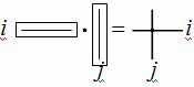

Let us emphasize once again that the product A·B makes sense if and only if the number of columns of the first factor is equal to the number of rows of the second, and the product produces a matrix whose number of rows is equal to the number of rows of the first factor, and the number of columns is equal to the number of columns of the second. You can check the result of multiplication using a special online calculator.

Example 7. Given matrices And . Find matrices C = A·B and D = B·A.
Solution. First of all, note that the product A·B exists because the number of columns of A is equal to the number of rows of B.

Example 8. Given a matrix . Find 3A 2 – 2A.
Solution.

.
; .
.
Let us note the following interesting fact.
As you know, the product of two non-zero numbers is not equal to zero. For matrices, a similar circumstance may not occur, that is, the product of non-zero matrices may turn out to be equal to the null matrix.